Fano Resonance: An Intuitive Explanation
Fano resonance is one of those line shapes that looks “too structured to be an accident”: a sharp peak accompanied by a dip, with an unmistakable asymmetry that refuses to be explained by a single Lorentzian. It shows up across physics — atomic spectra (auto-ionization), superconducting circuits, nanophotonics, and even cold-atom scattering — not because these systems are secretly the same, but because they share the same minimal interference mechanism: a narrow, long-lived resonance trying to coexist with a broad, slowly varying response. The catch is that — this is not “extra damping” or “a shifted resonance”; it is destructive interference that can drive the response all the way to zero at a specific frequency (an anti-resonance), even while the system is being driven. In this post, we attempt to build an intuition of the Fano resonance: two coupled, damped oscillators, one directly driven and one only excited indirectly through the coupling. For this, we resort to the coupled oscillator model.
Let us consider two oscillators with spring constants, $k_1$ and $k_2$, respectively. This two oscillators are connected via a third spring with spring constant $K$, as shown in Fig. 1. To avoid cluttering the equations with the $m$’s, we chose both masses to be the same and of unit magnitude, i.e., $m_1=m_2=1$ kg. Since the third spring (with spring-constant $K$) defines the strength of coupling between the two oscillators, we will refer to the coupling parameter between the two oscillators as $v_{12} \left( = \frac{K}{m_1}\right).$ From symmetry, $v_{12} = v_{21}.$ As usual, $\omega_1$ and $\omega_2$ (where $\omega_j= \sqrt{\frac{k_j}{m_j}}$ ) are the resonant frequencies of the oscillators, respectively. To keep things general, let’s define the damping constants as $\gamma_1$ and $\gamma_2$, respectively.
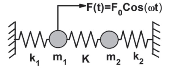
Fig. 1: Two masses are connected via two different springs. These two oscillators are coupled via a third spring with spring constant, $K$. The mass at the left is driven by a force with frequency $\omega$. Image credit: Google Images.
Now, the equation of motion for the two masses reads:
\[\ddot{x}_1 + \gamma_1 \dot{x}_1 +\omega_1^2 x_1 + v_{12} x_2 = F_0 \cos(\omega t),\] \[\ddot{x}_2 + \gamma_2 \dot{x}_1 +\omega_2^2 x_2 + v_{21} x_1 = 0,\]since the second mass is not being driven.
Characteristic equation for the eigenfrequencies of the system becomes (in the absence of loss, i.e. $\gamma_1 = \gamma_2 = 0$) –
\[(\omega^2-\omega_1^2) (\omega^2-\omega_2^2) - v_{12}^2 = 0.\]As the coupling $v_{12}$ ( as you remember, $v_{12}$ parameter defines the coupling between the two oscillators$ )$ becomes zero, the eigenfrequencies reduce to those of the uncoupled oscillators, this is some sort of sanity check of the calculations. (Food for thought: when $v_{12}^2>\omega_1 \omega_2$, then the first solution will be purely imaginary. That implies, no oscillation can persist in the first oscillator despite external excitation. This is the regime where Purcell factor becomes zero due to very strong coupling).
The response of the first oscillator, $x_1$ is shown in Fig. 2. Here, $\omega_1 = 1, \omega_2 = 1.25, \gamma_1 = 0.02, \gamma_2 = 0, v_{12} = 0.1$. As you can see, due to coupling between the oscillators, the response of the first oscillator has the spectral signature of the second oscillator as well. This asymmetric amplitude response of an oscillator is called the Fano resonance (near $\omega = \omega_2 = 1.25$).
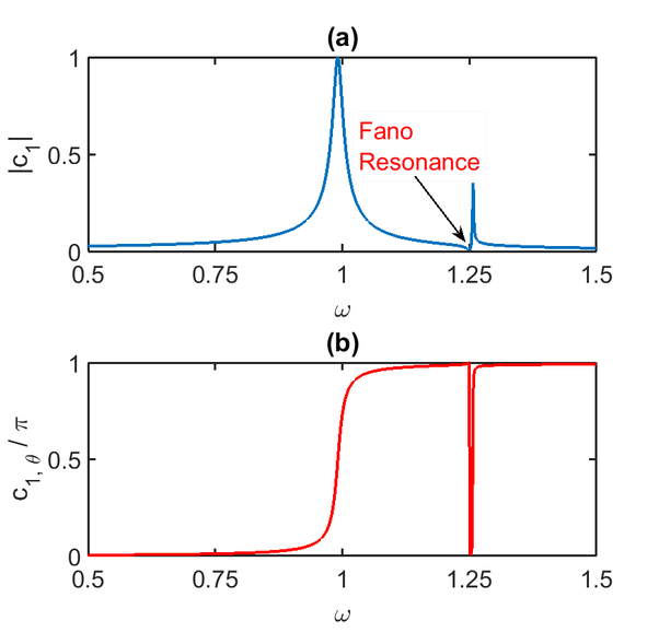
Fig. 2: (a) amplitude response, (b) phase of response, of the first oscillator due to an external force with frequency $\omega$. The parameters are, $\omega_1 = 1, \omega_2 = 1.25, \gamma_1 = 0.02, \gamma_2 = 0, v_{12} = 0.1$. As evident here, the asymmetric line shape, aka, the Fano resonance occurs at the resonance frequency of the second oscillator (i.e., $\omega = \omega_2 = 1.25$). (For careful readers: The first peak ($\omega \approx 1$) is a bit red-shifted from $ \omega = 1 $, this happens due to the presence of coupling constant, $v_{12} (\neq 0)$. If there were no coupling, the first peak would be exactly at $\omega = 1$.)
The interesting fact here is - the response of first oscillator contains a ‘null-response’ at the resonant frequency of the second oscillator (as you remember, $\omega_2 = 1.25$). This ‘null’ response is explained with Fig. 2(b), where you can see that as the phase of the first oscillator became $\pi$, after crossing its own resonant frequency, i.e. $\omega_1 = 1$, the phase then drops to zero at the resonant frequency of the second oscillator — an anti-resonance.
To get an intuition out of it: you will have Fano resonance whenever you have a slow-varying background and narrow-band resonance, altogether. The slow-varying background behaves like a continuum and it interacts with the bound-state having narrow spectrum. Due to this simple prerequisite, Fano line-shape is quite common in a myriad of phenomena ranging from Bose-Einstein condensates, auto-ionization, superconducting devices, to photonic crystals and many other photonic and solid-state systems.
I hope it now makes better sense intuitively, than it previously did.