Kramers’ theorem: If a system with total half-integer spin has time-reversal symmetry, then every energy eigenstate of the system has at least one partner with the same energy, i.e., the degeneracy is at least twofold.
In the following, I will delineate this concept with a concrete example. Let’s consider a portion of the band diagram for a spin-$\frac{1}{2}$ particle with time-reversal symmetry, shown in Fig. 1.
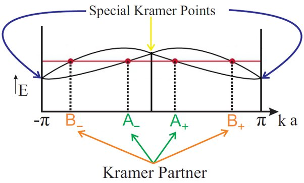
Fig. 1: Part of the band diagram for a spin-$\frac{1}{2}$ particle with time-reversal symmetry is shown. The points on the $\mathbf{k\cdot a}$ axis are color-coded to show the Kramers partners. Note that for a fixed energy (horizontal ‘red’ line) there are four energy eigenstates, and among the four states, $A_+$ is time-reversal partner of $A_-$, with equal but opposite $\mathbf{k\cdot a}$; likewise for $B_+$ and $B_-$. The special Kramers points are those who are their own time-reversal symmetric partner, and this leads to the degeneracy at those $\mathbf{k}$ points.
I would like to draw your attention to the special Kramer points as these points are their own time-reversal partner. Note that $k=\pi/a$ and $k=-\pi/a$ are the same point; and $k=0$ means quasimomentum is zero, thus it is invariant under time-reversal operation (if this sentence sounds fuzzy, please have a look at the Appendix). Since the degeneracy at those $\mathbf{k}$ points is protected by time-reversal symmetry, a global (i.e., time-independent) perturbation cannot break the degeneracy. Since a magnetic field breaks time-reversal symmetry, an applied magnetic field will lift the degeneracy at special Kramer points (please see the Appendixgelow if you would like to see an elaborated explanation of this sentence).
I will now try to elaborate the implications of the theorem and mention the points that I personally find fascinating. Since the theorem tells us that a Fermionic system with time-reversal symmetry (please see the Appendix below for a primer on time-reversal symmetry) is at least two-fold degenerate, one can make the following predictions about the system —
1. If there is an energy eigenstate, e.g., $\left|\varphi_\downarrow\right\rangle$, at $\mathbf{k\cdot a}=\zeta$ with energy $E$, in the band diagram of the system, then Kramers’ theorem guarantees that there is at least one more eigenstate with energy $E$ at $\mathbf{k\cdot a}=-\zeta$, with $\left|\varphi_\uparrow\right\rangle$. Note that funny thing happens at $\mathbf{k\cdot a}=0~\mathrm{and}~\pi$— the energy eigenstates are at least two-fold degenerate at those points. The degeneracy at those points is due to the fact that $\mathbf{k\cdot a}=0~\mathrm{and}~\pi$ are their own time-reversal symmetric partner, in the first Brillouin zone. This conspires them to have degenerate energy eigenstates with the same $\mathbf{k}\cdot\mathbf{a}$, at each of these points ($\mathbf{k\cdot a}=0,~\pi$).
2. If any perturbation to the system does not break the time-reversal symmetry, the degeneracy at $\mathbf{k\cdot a}=0~\mathrm{and}~\pi$ remains intact. This leads to the next point.
3. The theorem holds so long as the time-reversal symmetry is intact, however any perturbation that breaks the time-reversal symmetry may lead to the lifting of degeneracy — the eigenstates at $\mathbf{k\cdot a}=0~ \mathrm{and}~\pi $ are no longer guaranteed to have degeneracy. In principle, a broken time-reversal symmetric system may have degenerate eigenstates, however that degeneracy could be lifted by any small perturbation, e.g., small disorder.
4. There is another interesting aspect of this theorem pertaining to superconductivity. As you might know, superconductors form a macroscopic wavefunction due to the pairing of electrons of opposite spins — forming bosons — called Cooper pairs. Philip Anderson argued that the superconductivity can survive even in the presence of disorder, this is sometimes called Dirty Superconductor Theorem [Anderson1959]. His argument was as follows: although the presence of disorder will distort the Fermi surface, however for every electron with spin up $\left|\Psi_\uparrow\right\rangle,$ at Fermi surface, there will be another time-reversal symmetric partner with spin down$\left|\Psi_\downarrow\right\rangle,$ thus they can always form a Cooper pair. Although the superconductor with disorder will have a smaller critical temperature, the formation of Cooper pair is robust so long as the disorder does not break the time-reversal symmetry.
(Bonus: Superconductivity remains intact in the presence of spin-orbit interaction (SOI) — since spin-orbit interaction preserves time-reversal symmetry and spin is not a good quantum number in the presence of SOI. For spin-orbit coupled electrons, the electrons can still pair up with their Kramers pair having the same energy, and form Cooper pairs — thus keeping the superconductivity intact. )
I personally believe that the beauty of the theorem is that — with this theorem, one can learn a lot about a system with only two pieces of information, namely 1. the system has total half-integer spin, 2. the time-reversal symmetry is preserved. And with these information, one can predict how the system would respond to a given perturbation, without doing any explicit calculation. Finally, the argument of Phil Anderson on the robustness of superconductivity, in the presence of disorder is mind-boggling.
Appendix: Time-reversal Symmetry
Time-reversal symmetry is exactly what it sounds like — the system remains invariant if we reverse the ‘arrow of time’. Before a rigorous treatment of the concept, let us try to build some intuition.
The time-reversal symmetry operator $\mathcal{T}$ involves the following transformation
\[\mathcal{T}:~t\rightarrow-t.\]Since it reverses the sign of time $t$, the position vector $\mathbf{x}$ will remain the same (space and time are independent), although velocity will pick-up a minus sign if we perform a time-reversal operation:
\[\mathcal{T}:~\left( {\mathbf{ v } = \frac{d}{{dt}}\mathbf{ x}} \right) \rightarrow \left( {\mathbf{v'} = \frac{d}{{d\left( { - t} \right)}}\mathbf{ x } = - \mathbf{ v } } \right).\]By the same argument, electric current density $\mathbf{j}=nq\mathbf{v}$ will pick-up minus sign since charge $q$ is invariant under the operation of $\mathcal{T}$.
Now we can understand why we call $\mathbf{k\cdot a}=0~\mathrm{and}~\pi$ points as time-reversal-symmetric points in the Brillouin zone: although $\hbar k$ is quasi-momentum, we can associate them with velocity and at $\mathbf{k\cdot a}=0$ and $\pi$, these points map onto themselves since $\mathbf{k}=0\rightarrow\mathbf{k}=0 $ and $\mathbf{k\cdot a}=\pi\rightarrow\mathbf{k\cdot a}=-\pi$ (which is the same point as $\pi$). Since these points are their own time-reversal symmetric partner, they cannot get rid of the degeneracy, at these points, in a system with $\mathcal{T} $ symmetry.
The usual variables in classical electrodynamics are electric field $\mathbf{E}$ and electric displacement $\mathbf{D}=\widehat{\epsilon}\mathbf{E}$ where $\widehat{\epsilon}$ is the dielectric tensor that is usually time-independent. Since $\mathrm{div}~\mathbf{D}=4\pi\rho$, the displacement vector $\mathbf{D}$ does not change under $\mathcal{T}$ and electric field is also invariant. The reason these two parameters are mentioned is — I would like to show that magnetic field does pick-up a minus sign and the application of magnetic field breaks time-reversal symmetry of an otherwise time-reversal symmetric system. It can be seen as follows:
\[\mathcal{T}:~\left(\mathrm{rot}~\mathbf{B} = \frac{{4\pi }}{c} \mathbf{j} + \frac{1}{c}\frac{\partial }{{\partial t}}\mathbf{E}\right)\to \left(\mathrm{rot} \left(\mathbf{B}\right) = -\frac{{4\pi }}{c} \mathbf{j} + \frac{1}{c}\frac{\partial }{{\partial (-t)}}\mathbf{E}\right)\to \left(\mathrm{rot} \left(-\mathbf{B}\right) = \frac{{4\pi }}{c} \mathbf{j} + \frac{1}{c}\frac{\partial }{{\partial t}}\mathbf{E}\right).\]Since both the current density $\mathbf{j}$ and time $t$ pick-up minus signs under time-reversal symmetry while electric field $\mathbf{E}$ remains invariant, thus magnetic field $\mathbf{B}$ has to pick-up minus sign, in order to preserve the equality (the equality has to be preserved since Maxwell’s equations are Lorentz invariant). Thus an easy way to break time-reversal symmetry is to apply a magnetic field and this will subsequently lift the stringent requirement of having degeneracy at $\mathbf{k\cdot a}=0~\mathrm{and}~\pi$ points, in the band structure of a Fermionic system.
Now that we have some intuition of the $\mathcal{T}$ symmetry, we will explore it in the realm of quantum mechanics.
Classically, $\mathcal{T}$ involves a sign reversal of time $t$. However, in quantum mechanics the full $\mathcal{T}$ operator involves two simultaneous operations:
- $t \to -t,$
- $i \to -i.$ (Side note: the above substitutions have some deep and profound implications in $\mathcal{PT}-$symmetric systems that host real spectrum for non-Hermitian Hamiltonians [Bender1998].) The justification of the replacement $i\to-i$ has its root on the preconceived idea that energy cannot change sign under the operation of $\mathcal{T}$.
For a spin-$\frac{1}{2}$ system, it can be argued and proved that the operator $\mathcal{T}$ takes the form $\mathcal{T}=U_T\theta$, where $U_T$ is a unitary matrix and $\theta$ is complex-conjugation operator ($\theta^2=\mathbb{1}$). Since transformation via $\mathcal{T}$ will flip the sign of the spinor for a spin-$\frac{1}{2}$ particle, we have the following relations
\[\mathcal{T}{\sigma _x}{\mathcal{T}^{ - 1}} = - {\sigma _x},\qquad\mathcal{T}{\sigma _y}{\mathcal{T}^{ - 1}} = - {\sigma _y},\qquad\mathrm{and}~\mathcal{T}{\sigma _z}{\mathcal{T}^{ - 1}} = - {\sigma _z}.\]The only form of $U_T$ that satisfies the above three relations is $U_T=\sigma_y\exp(i\varphi)$ where $\varphi$ is a gauge-dependent phase and we will not bother about it much.
Although two consecutive operations of $\mathcal{T}$ are supposed to restore the system back to its original configuration, classically. It is not necessarily the case for a spin-$\frac{1}{2} $ particle — in fact it picks up a minus sign. It was Eugene Wigner who used $\mathcal{T}^2=-1$ to prove Kramer’s degeneracy [Wigner1932], however this property has been under the spotlight since the rejuvenation of topological matter.
Further Reading
- [Anderson1959] Anderson, P.W., Theory of dirty superconductors. Journal of Physics and Chemistry of Solids, 11, pp.26-30 (1959).
-
[Bender1998] Bender, C.M. and Boettcher, S., Real spectra in non-Hermitian Hamiltonians having $\mathcal{P T}$ symmetry. Physical Review Letters, 80, p.5243 (1998).
- [Wigner1932] Eugene P. Wigner. Uber die Operation der Zeitumkehr in der Quantenmechanik. Nachrichten der Gesellschaft der Wissenschaften zu Gottingen Mathematisch Physikalische Klasse, pp. 546–559, (1932). (Although the paper by Wigner is in German, the proof in English can be found in the Section-2 of this paper by Brian Roberts).